AiiDA basics¶

This module will give you a first taste of some of the features of AiiDA, and help you familiarize with the verdi command-line interface (CLI), as well as AiiDA’s IPython shell.

Important

Before starting this tutorial, make sure you have watched the demonstration on working with your virtual machine. Also remember to run workon aiida in any new terminal, in order to enter the correct virtual environment, otherwise the verdi command will not be available.

The verdi command supports tab-completion: In the terminal, type verdi, followed by a space and press the ‘Tab’ key twice to show a list of all the available sub commands.
For help on verdi or any of its subcommands, simply append the --help/-h flag, e.g.:
```
$ verdi quicksetup -h
```

More details on verdi can be found in the online documentation.

Provenance¶

Before we continue, we need to briefly introduce one of the most important concepts for AiiDA: provenance. An AiiDA database does not only contain the results of your calculations, but also their inputs and each step that was executed to obtain them. All of this information is stored in the form of a directed acyclic graph (DAG). As an example, Fig. 1 shows the provenance of the calculations of the first part of this tutorial.

../../_images/basics_workchain_graph.png

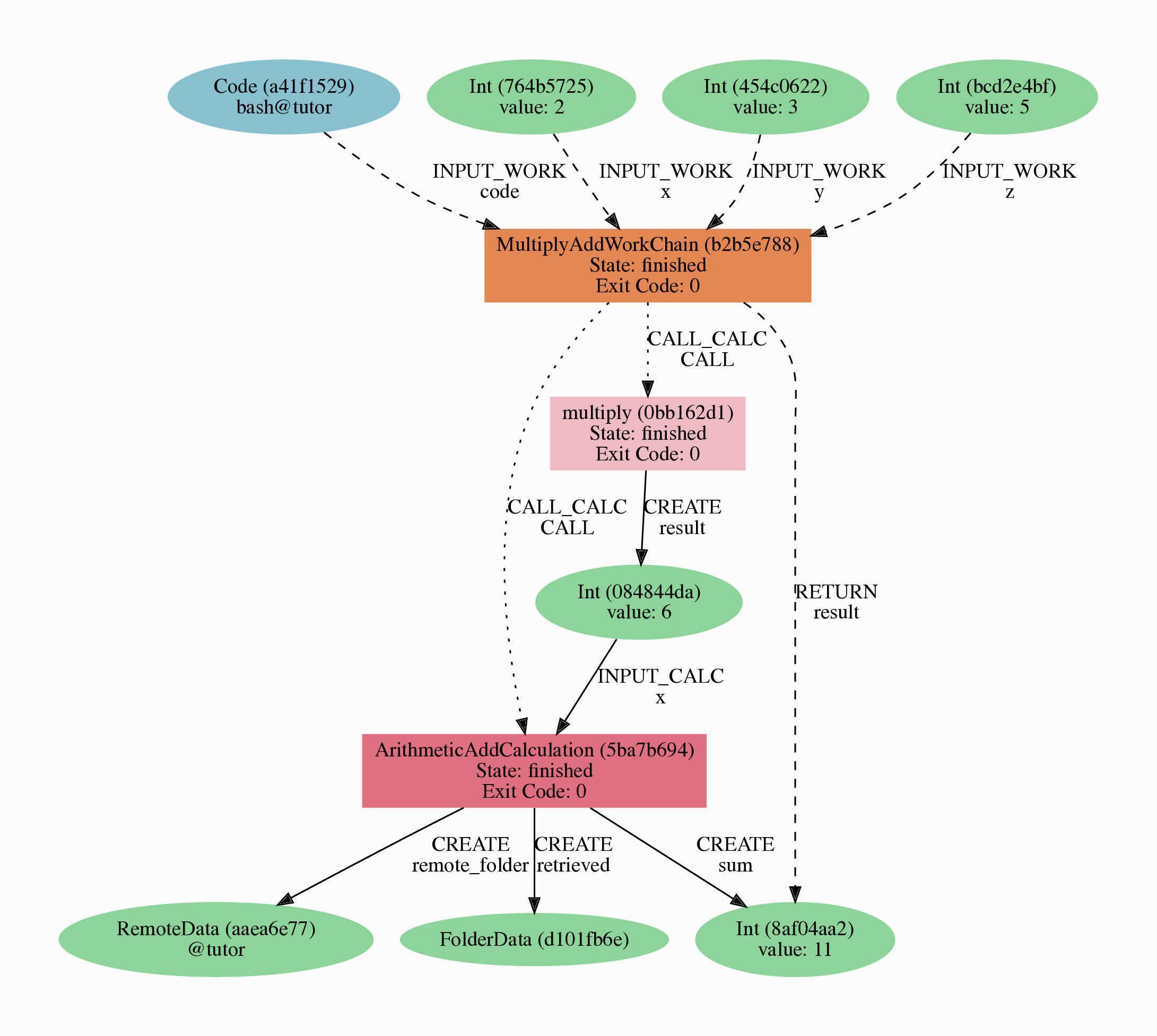
Fig. 1 Provenance Graph of a basic AiiDA WorkChain.¶

In the provenance graph, you can see different types of nodes represented by different shapes. The green ellipses are Data nodes, the blue ellipse is a Code node, and the rectangles represent processes, i.e. the calculations performed in your workflow.

The provenance graph allows us to not only see what data we have, but also how it was produced. During this basic tutorial we will first be using AiiDA to generate the provenance graph in Fig. 1, step by step.

Data nodes¶

Before running any calculations, let’s create and store a data node. AiiDA ships with an interactive IPython shell that has many basic AiiDA classes pre-loaded. To start the IPython shell, simply type in the terminal:

$ verdi shell

AiiDA implements data node types for the most common types of data (int, float, str, etc.), which you can extend with your own (composite) data node types if needed. For this tutorial, we’ll keep it very simple, and start by initializing an Int node and assigning it to the {}node variable:

In [1]: node = Int(2)

Note

Commands you have to execute in the bash terminal or the IPython shell can be clearly distinguished via the corresponding prompts and different box colors.

We can check the contents of the node variable like this:

In [2]: node
Out[2]: <Int: uuid: eac48d2b-ae20-438b-aeab-2d02b69eb6a8 (unstored) value: 2>

Quite a bit of information on our freshly created node is returned:

The data node is of the type Int
The node has the universally unique identifier (UUID) eac48d2b-ae20-438b-aeab-2d02b69eb6a8
The node is currently not stored in the database (unstored)
The integer value of the node is 2

Let’s store the node in the database:

In [3]: node.store()
Out[3]: <Int: uuid: eac48d2b-ae20-438b-aeab-2d02b69eb6a8 (pk: 1) value: 2>

As you can see, the data node has now been assigned a primary key (PK), a number that identifies the node in your database (pk: 1). The PK and UUID both reference the node with the only difference that the PK is unique for your local database only, whereas the UUID is a globally unique identifier and can therefore be used between different databases. Use the PK only if you are working within a single database, i.e. in an interactive session and the UUID in all other cases.

Important

The PK numbers shown throughout this first tutorial assume that you start from a completely empty database. It is possible that the nodes’ PKs will be different for your database!

The UUIDs are generated randomly and are therefore guaranteed to be different for nodes created during the tutorial.

Next, let’s leave the IPython shell by typing exit() and then enter. Back in the terminal, use the verdi command line interface (CLI) to check the data node we have just created:

$ verdi node show 1

This prints something like the following:

Property     Value
-----------  ------------------------------------
type         Int
pk           1
uuid         eac48d2b-ae20-438b-aeab-2d02b69eb6a8
label
description
ctime        2020-05-13 08:58:15.193421+00:00
mtime        2020-05-13 08:58:40.976821+00:00

Once again, we can see that the node is of type Int, has PK = 1, and UUID = eac48d2b-ae20-438b-aeab-2d02b69eb6a8. Besides this information, the verdi node show command also shows the (empty) label and description, as well as the time the node was created (ctime) and last modified (mtime).

Note

AiiDA already provides many standard data types, but you can also create your own.

Calculation functions¶

Once your data is stored in the database, it is ready to be used for some computational task. For example, let’s say you want to multiply two Int data nodes. The following Python function:

def multiply(x, y):
    return x * y

will give the desired result when applied to two Int nodes, but the calculation will not be stored in the provenance graph. However, we can use a Python decorator provided by AiiDA to automatically make it part of the provenance graph. Start up the AiiDA IPython shell again using verdi shell and execute the following code snippet:

In [1]: from aiida.engine import calcfunction
   ...:
   ...: @calcfunction
   ...: def multiply(x, y):
   ...:     return x * y

This converts the multiply function into an AiIDA calculation function, the most basic execution unit in AiiDA. Next, load the Int node you have created in the previous section using the load_node function and the PK of the data node:

In [2]: x = load_node(pk=1)

Of course, we need another integer to multiply with the first one. Let’s create a new Int data node and assign it to the variable y:

In [3]: y = Int(3)

Now it’s time to multiply the two numbers!

In [4]: multiply(x, y)
Out[4]: <Int: uuid: 42541d38-1fb3-4f60-8122-ab8b3e723c2e (pk: 4) value: 6>

Success! The calcfunction-decorated multiply function has multiplied the two Int data nodes and returned a new Int data node whose value is the product of the two input nodes. Note that by executing the multiply function, all input and output nodes are automatically stored in the database:

In [5]: y
Out[5]: <Int: uuid: 7865c8ff-f243-4443-9233-dd303a9be3c5 (pk: 2) value: 3>

We had not yet stored the data node assigned to the y variable, but by providing it as an input argument to the multiply function, it was automatically stored with PK = 2. Similarly, the returned Int node with value 6 has been stored with PK = 4.

Let’s once again leave the IPython shell with exit() and look for the process we have just run using the verdi CLI:

$ verdi process list

The returned list will be empty, but don’t worry! By default, verdi process list only returns the active processes. If you want to see all processes (i.e. also the processes that are terminated), simply add the -a option:

$ verdi process list -a

You should now see something like the following output:

  PK  Created    Process label    Process State    Process status
----  ---------  ---------------  ---------------  ----------------
   3  1m ago     multiply         ⏹ Finished [0]

Total results: 1

Info: last time an entry changed state: 1m ago (at 09:01:05 on 2020-05-13)

We can see that our multiply calcfunction was created 1 minute ago, assigned the PK 3, and has Finished.

As a final step, let’s have a look at the provenance of this simple calculation. The provenance graph can be automatically generated using the verdi CLI. Let’s generate the provenance graph for the multiply calculation function we have just run with PK = 3:

$ verdi node graph generate 3

Note

Remember that the PK of the calculation function can be different for your database.

The command will write the provenance graph to a .pdf file. You can open this file on the Amazon virtual machine by using evince:

$ evince 3.dot.pdf

If X-forwarding has been setup correctly, the provenance graph should appear on your local machine. In case the ssh connection is too slow, copy the file via scp to your local machine. To do so, if you are using Linux/Mac OS X, you can type in your local machine:

$ scp aiidatutorial:<path_to_the_graph_pdf> <local_folder>

and then open the file.

Note

You can also use the jupyter notebook setup explained (TODO: FIX LINK) to download files. Note that while Firefox will display the PDF directly in the browser Chrome and Safari block viewing PDFs from jupyter notebook servers - with these browsers, you will need to tick the checkbox next to the PDF and download the file.

Alternatively, you can use graphical software to achieve the same, for instance: on Windows: WinSCP; on a Mac: Cyberduck; on Linux Ubuntu: using the ‘Connect to server’ option in the main menu after clicking on the desktop.

It should look something like the graph shown in Fig. 2.

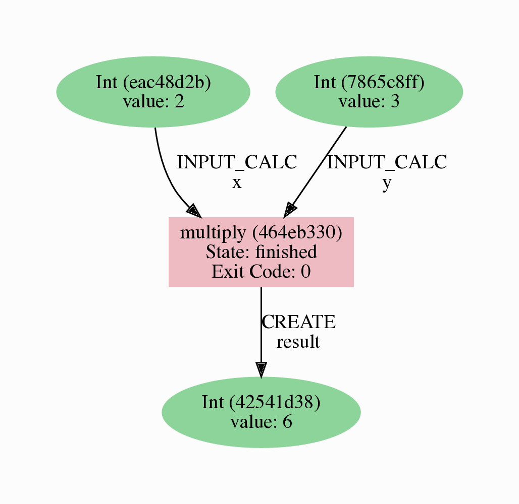
Fig. 2 Provenance graph of the multiply calculation function.¶

CalcJobs¶

When running calculations that require an external code or run on a remote machine, a simple calculation function is no longer sufficient. For this purpose, AiiDA provides the CalcJob process class. To run a CalcJob, you need to set up two things: a code that is going to implement the desired calculation and a computer for the calculation to run on. Let’s begin by setting up the computer using the verdi computer subcommand:

$ verdi computer setup -L tutor -H localhost -T local -S direct -w `echo $PWD/work` -n
$ verdi computer configure local tutor --safe-interval 5 -n

The first commands sets up the computer with the following options:

label (-L): tutor
hostname (-H): localhost
transport (-T): local
scheduler (-S): direct
work-dir (-w): The work subdirectory of the current directory

The second command configures the computer with a minimum interval between connections (--safe-interval) of 5 seconds. For both commands, the non-interactive option (-n) is added to not prompt for extra input.

Next, let’s set up the code we’re going to use for the tutorial:

$ verdi code setup -L add --on-computer --computer=tutor -P arithmetic.add --remote-abs-path=/bin/bash -n

This command sets up a code with label add on the computer tutor, using the plugin arithmetic.add.

A typical real-world example of a computer is a remote supercomputing facility. Codes can be anything from a Python script to powerful ab initio codes such as Quantum ESPRESSO or machine learning tools like Tensorflow. Let’s have a look at the codes that are available to us:

$ verdi code list
# List of configured codes:
# (use 'verdi code show CODEID' to see the details)
* pk 5 - add@tutor

You can see a single code add@tutor, with PK = 5, in the printed list. This code allows us to add two integers together. The add@tutor identifier indicates that the code with label add is run on the computer with label tutor. To see more details about the computer, you can use the following verdi command:

$ verdi computer show tutor
Computer name:     tutor
 * PK:             1
 * UUID:           b9ecb07c-d084-41d7-b862-a2b1f02722c5
 * Description:
 * Hostname:       localhost
 * Transport type: local
 * Scheduler type: direct
 * Work directory: /Users/mbercx/epfl/tutorials/my_tutor/work
 * Shebang:        #!/bin/bash
 * mpirun command: mpirun -np {tot_num_mpiprocs}
 * prepend text:
 # No prepend text.
 * append text:
 # No append text.

We can see that the Work directory has been set up as the work subdirectory of the current directory. This is the directory in which the calculations running on the tutor computer will be executed.

Note

You may have noticed that the PK of the tutor computer is 1, same as the Int node we created at the start of this tutorial. This is because different entities, such as nodes, computers and groups, are stored in different tables of the database. So, the PKs for each entity type are unique for each database, but entities of different types can have the same PK within one database.

Let’s now start up the verdi shell again and load the add@tutor code using its label:

In [1]: code = load_code(label='add')

Every code has a convenient tool for setting up the required input, called the builder. It can be obtained by using the get_builder method:

In [2]: builder = code.get_builder()

Using the builder, you can easily set up the calculation by directly providing the input arguments. Let’s use the Int node that was created by our previous calcfunction as one of the inputs and a new node as the second input:

In [3]: builder.x = load_node(pk=4)
   ...: builder.y = Int(5)

In case that your nodes’ PKs are different and you don’t remember the PK of the output node from the previous calculation, check the provenance graph you generated earlier and use the UUID of the output node instead:

In [3]: builder.x = load_node(uuid='42541d38')
   ...: builder.y = Int(5)

Note that you don’t have to provide the entire UUID to load the node. As long as the first part of the UUID is unique within your database, AiiDA will find the node you are looking for.

Note

One nifty feature of the builder is the ability to use tab completion for the inputs. Try it out by typing builder. + <TAB> in the verdi shell.

To execute the CalcJob, we use the run function provided by the AiiDA engine:

In [4]: from aiida.engine import run
   ...: run(builder)

Wait for the process to complete. Once it is done, it will return a dictionary with the output nodes:

Out[4]:
{'sum': <Int: uuid: 7d5d781e-8f17-498a-b3d5-dbbd3488b935 (pk: 8) value: 11>,
'remote_folder': <RemoteData: uuid: 888d654a-65fb-4da0-b3bc-d63f0374f274 (pk: 9)>,
'retrieved': <FolderData: uuid: 4733aa78-2e2f-4aeb-8e09-c5cfb58553db (pk: 10s)>}

Besides the sum of the two Int nodes, the calculation function also returns two other outputs: one of type RemoteData and one of type FolderData. See the topics section on calculation jobs for more details. Now, exit the IPython shell and once more check for all processes:

$ verdi process list -a

You should now see two processes in the list. One is the multiply calcfunction you ran earlier, the second is the ArithmeticAddCalculation CalcJob that you have just run. Grab the PK of the ArithmeticAddCalculation, and generate the provenance graph. The result should look like the graph shown in Fig. 3.

$ verdi node graph generate 7

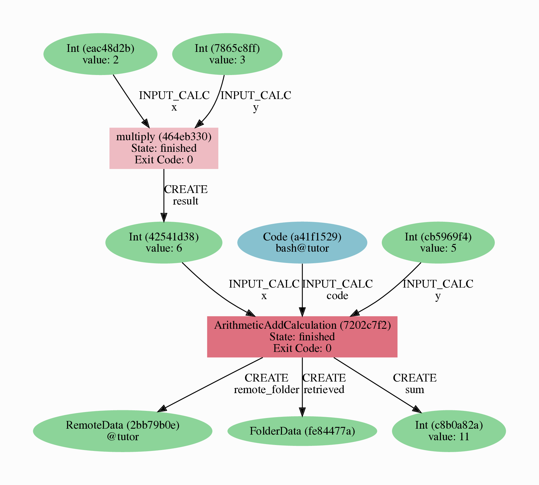
Fig. 3 Provenance graph of the ArithmeticAddCalculation CalcJob, with one input provided by the output of the multiply calculation function.¶

You can see more details on any process, including its inputs and outputs, using the verdi shell:

$ verdi process show 7

Submitting to the daemon¶

When we used the run command in the previous section, the IPython shell was blocked while it was waiting for the CalcJob to finish. This is not a problem when we’re simply multiplying two numbers, but if we want to run multiple calculations that take hours or days, this is no longer practical. Instead, we are going to submit the CalcJob to the AiiDA daemon. The daemon is a program that runs in the background and manages submitted calculations until they are terminated. Let’s first check the status of the daemon using the verdi CLI:

$ verdi daemon status

If the daemon is running, the output will be something like the following:

Profile: tutorial
Daemon is running as PID 96447 since 2020-05-22 18:04:39
Active workers [1]:
  PID    MEM %    CPU %  started
-----  -------  -------  -------------------
96448    0.507        0  2020-05-22 18:04:39
Use verdi daemon [incr | decr] [num] to increase / decrease the amount of workers

In this case, let’s stop it for now:

$ verdi daemon stop

Next, let’s submit the CalcJob we ran previously. Start the verdi shell and execute the Python code snippet below. This follows all the steps we did previously, but now uses the submit function instead of run:

In [1]: from aiida.engine import submit
   ...:
   ...: code = load_code(label='add')
   ...: builder = code.get_builder()
   ...: builder.x = load_node(pk=4)
   ...: builder.y = Int(5)
   ...:
   ...: submit(builder)

When using submit the calculation job is not run in the local interpreter but is sent off to the daemon and you get back control instantly. Instead of the result of the calculation, it returns the node of the CalcJob that was just submitted:

Out[1]: <CalcJobNode: uuid: e221cf69-5027-4bb4-a3c9-e649b435393b (pk: 12) (aiida.calculations:arithmetic.add)>

Let’s exit the IPython shell and have a look at the process list:

$ verdi process list

You should see the CalcJob you have just submitted, with the state Created:

  PK  Created    Process label             Process State    Process status
----  ---------  ------------------------  ---------------  ----------------
  12  13s ago    ArithmeticAddCalculation  ⏹ Created

Total results: 1

Info: last time an entry changed state: 13s ago (at 09:06:57 on 2020-05-13)

The CalcJob process is now waiting to be picked up by a daemon runner, but the daemon is currently disabled. Let’s start it up (again):

$ verdi daemon start

Now you can either use verdi process list to follow the execution of the CalcJob, or watch its progress:

$ verdi process watch 12

Let’s wait for the CalcJob to complete (state changes to “finished”). Quit the watch command (Ctrl+C) and use verdi process list -a to see all processes we have run so far:

  PK  Created    Process label             Process State    Process status
----  ---------  ------------------------  ---------------  ----------------
   3  6m ago     multiply                  ⏹ Finished [0]
   7  2m ago     ArithmeticAddCalculation  ⏹ Finished [0]
  12  1m ago     ArithmeticAddCalculation  ⏹ Finished [0]

Total results: 3

Info: last time an entry changed state: 14s ago (at 09:07:45 on 2020-05-13)

Workflows¶

So far we have executed each process manually. AiiDA allows us to automate these steps by linking them together in a workflow, whose provenance is stored to ensure reproducibility. For this tutorial we have prepared a basic WorkChain that is already implemented in aiida-core. You will see the details of this code in the section on (TODO: FIX LINK).

Note

Besides WorkChain’s, workflows can also be implemented as work functions. These are ideal for workflows that are not very computationally intensive and can be easily implemented in a Python function.

Let’s run the WorkChain above! Start up the verdi shell and load the MultiplyAddWorkChain using the WorkflowFactory:

In [1]: MultiplyAddWorkChain = WorkflowFactory('arithmetic.multiply_add')

The WorkflowFactory is a useful and robust tool for loading workflows based on their entry point, e.g. 'arithmetic.multiply_add' in this case. Similar to a CalcJob, the WorkChain input can be set up using a builder:

In [2]: builder = MultiplyAddWorkChain.get_builder()
   ...: builder.code = load_code(label='add')
   ...: builder.x = Int(2)
   ...: builder.y = Int(3)
   ...: builder.z = Int(5)

Once the WorkChain input has been set up, we submit it to the daemon using the submit function from the AiiDA engine:

In [3]: from aiida.engine import submit
   ...: submit(builder)

Now quickly leave the IPython shell and check the process list:

$ verdi process list -a

Depending on which step the workflow is running, you should get something like the following:

  PK  Created    Process label             Process State    Process status
----  ---------  ------------------------  ---------------  ------------------------------------
   3  7m ago     multiply                  ⏹ Finished [0]
   7  3m ago     ArithmeticAddCalculation  ⏹ Finished [0]
  12  2m ago     ArithmeticAddCalculation  ⏹ Finished [0]
  19  16s ago    MultiplyAddWorkChain      ⏵ Waiting        Waiting for child processes: 22
  20  16s ago    multiply                  ⏹ Finished [0]
  22  15s ago    ArithmeticAddCalculation  ⏵ Waiting        Waiting for transport task: retrieve

Total results: 6

Info: last time an entry changed state: 0s ago (at 09:08:59 on 2020-05-13)

We can see that the MultiplyAddWorkChain is currently waiting for its child process, the ArithmeticAddCalculation, to finish. Check the process list again for all processes (You should know how by now!). After about half a minute, all the processes should be in the Finished state.

We can now generate the full provenance graph for the WorkChain with:

$ verdi node graph generate 19

Open the generated pdf file using evince. Look familiar? The provenance graph should be similar to the one we showed at the start of this tutorial (Fig. 4).

Fig. 4 Final provenance Graph of the basic AiiDA tutorial.¶

(Optional section) Comments¶

AiiDA offers the possibility to attach comments to a any node, in order to be able to remember more easily its details. Node with UUID prefix ce81c420 should have no comments, but you can add a very instructive one by typing in the terminal:

$ verdi node comment add "vc-relax of a BaTiO3 done with QE pw.x" -N <IDENTIFIER>

Now, if you ask for a list of all comments associated to that calculation by typing:

$ verdi node comment show <IDENTIFIER>

the comment that you just added will appear together with some useful information such as its creator and creation date. We let you play with the other options of verdi node comment command to learn how to update or remove comments.

AiiDA Tutorials

AiiDA basics¶

Provenance¶

Data nodes¶

Calculation functions¶

CalcJobs¶

Submitting to the daemon¶

Workflows¶

(Optional section) Comments¶